
JR: James Hansen’s recent work on attributing climate extremes to global warming is very important. That’s because off-the-charts extreme weather — along with its impact on food production — is how most Americans and indeed most homo sapiens are likely to experience the negative impacts of climate change for the foreseeable future. So it’s no surprise that it has come under attack.
NASA’s Gavin Schmidt has an excellent explanation of why Hansen’s analysis is so relevant and why some of his critics are so wrong. The bottom line: The critics apparently think climate impacts are linear — a small change always has a small incremental impact — whereas reality makes clear that the impacts are non-linear and have potentially dangerous thresholds. There is a straw that breaks the climate’s back, and we would appear to be fast approaching it.
There has been a lot of discussion related to the Hansen et al (2012, PNAS) paper and the accompanying op-ed in the Washington Post last week. But in this post, I’ll try and make the case that most of the discussion has not related to the actual analysis described in the paper, but rather to proxy arguments for what people think is ‘important’.
The basic analysis
What Hansen et al have done is actually very simple. If you define a climatology (say 1951-1980, or 1931-1980), calculate the seasonal mean and standard deviation at each grid point for this period, and then normalise the departures from the mean, you will get something that looks very much like a Gaussian ‘bell-shaped’ distribution. If you then plot a histogram of the values from successive decades, you will get a sense for how much the climate of each decade departed from that of the initial baseline period.

The shift in the mean of the histogram is an indication of the global mean shift in temperature, and the change in spread gives an indication of how regional events would rank with respect to the baseline period. (Note that the change in spread shouldn’t be automatically equated with a change in climate variability, since a similar pattern would be seen as a result of regionally specific warming trends with constant local variability). [Now combine] this figure … with the change in areal extent of warm temperature extremes:
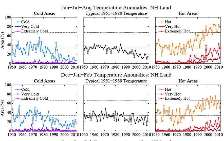
[These] are the main results that lead to Hansen et al’s conclusion that:
“hot extreme[s], which covered much less than 1% of Earth’s surface during the base period, now typically [cover] about 10% of the land area. It follows that we can state, with a high degree of confidence, that extreme anomalies such as those in Texas and Oklahoma in 2011 and Moscow in 2010 were a consequence of global warming because their likelihood in the absence of global warming was exceedingly small.”
What this shows first of all is that extreme heat waves, like the ones mentioned, are not just “black swans” – i.e. extremely rare events that happened by “bad luck”. They might look like rare unexpected events when you just focus on one location, but looking at the whole globe, as Hansen et al. did, reveals an altogether different truth: Such events show a large systematic increase over recent decades and are by no means rare any more.
At any given time, they now cover about 10% of the planet. What follows is that the likelihood of 3 sigma+ temperature events (defined using the 1951-1980 baseline mean and sigma) has increased by such a striking amount that attribution to the general warming trend is practically assured. We have neither long enough nor good enough observational data to have a perfect knowledge of the extremes of heat waves given a steady climate, and so no claim along these lines can ever be for 100% causation, but the change is large enough to be classically ‘highly significant’.
The point I want to stress here is that the causation is for the metric “a seasonalmonthlyanomaly greater than 3 sigma above the mean”.
This metric comes follows on from work that Hansen did a decade ago exploring the question of what it would take for people to notice climate changing, since they only directly experience the weather (Hansen et al, 1998) (pdf), and is similar to metrics used by Pall et al and other recent papers on the attribution of extremes. It is closely connected to metrics related to return times (i.e. if areal extent of extremely hot anomalies in any one summer increases by a factor of 10, then the return time at an average location goes from 1 in 330 years to 1 in 33 years).
A similar conclusion to Hansen was reached by Rahmstorf and Coumou (2011) (pdf)) but for a related but different metric: the probability of record-breaking events rather than 3-sigma events. For the Moscow heat record of July 2010, they found that the probability of a record had increased five-fold due to the local climatic warming trend, as compared to a stationary climate (see our previous articles The Moscow warming hole and On record-breaking extremes for further discussion). An similarly concluded extension of this analysis to the whole globe is currently in review.
There have been been some critiques of Hansen et al. worth addressing – Marty Hoerling’s statements in the NY Times story referring to his work (Dole et al, 2010) and Hoerling et al, (submitted) on attribution of the Moscow and Texas heat-waves, and a blog post by Cliff Mass of the U. of Washington. *
*We can just skip right past the irrelevant critique from Pat Michaels – someone well-versed in misrepresenting Hansen’s work – since it consists of proving wrong a claim (that US drought is correlated to global mean temperature) that appears nowhere in the paper – even implicitly. This is like criticising a diagnosis of measles by showing that your fever is not correlated to the number of broken limbs.
The metrics that Hoerling and Mass use for their attribution calculations are the absolute anomaly above climatology. So if a heat wave is 7ºC above the average summer, and since global warming could have contributed 1 or 2ºC (depending on location, season etc.), the claim is that only 1/7th or 2/7th’s of the anomaly is associated with climate change, and that the bulk of the heat wave is driven by whatever natural variability has always been important (say, La Niña or a blocking high).
But this Hoerling-Mass ratio is a very different metric than the one used by Hansen, Pall, Rahmstorf & Coumou, Allen and others, so it isn’t fair for Hoerling and Mass to claim that the previous attributions are wrong – they are simply attributing a different thing. This only rarely seems to be acknowledged. We discussed the difference between those two types of metrics previously in Extremely hot. There we showed that the more extreme an event is, the more does the relative likelihood increase as a result of a warming trend.
So which metric ‘matters’ more? and are there other metrics that would be better or more useful?
A question of values
What people think is important varies enormously, and as the French say ‘Les goûts et les couleurs ne se discutent pas’ (Neither tastes nor colours are worth arguing about). But is the choice of metric really just a matter of opinion? I think not.
Why do people care about extreme weather events? Why for instance is a week of 1ºC above climatology uneventful, yet a day with a 7ºC anomaly is something to be discussed on the evening news? It is because the impacts of a heat wave are very non-linear. The marginal effect of an additional 1ºC on top of 6ºC on many aspects of a heat wave (on health, crops, power consumption etc.) is much more than the effect of the first 1ºC anomaly. There are also thresholds – temperatures above which systems will cease to work at all. One would think this would be uncontroversial. Of course, for some systems not near any thresholds and over a small enough range, effects can be approximated as linear, but at some point that will obviously break down – and the points at which it does are clearly associated with extremes that with the most important impacts.
Only if we assume that the all responses are linear, can there be a clear separation between the temperature increases caused by global warming and the internal variability over any season or period, and the attribution of effects scales like the Hoerling-Mass ratio. But even then the “fraction of the anomaly due to global warming” is somewhat arbitrary because it depends on the chosen baseline for defining the anomaly – is it the average July temperature, or typical previous summer heat waves (however defined), or the average summer temperature, or the average annual temperature? In the latter (admittedly somewhat unusual) choice of baseline, the fraction of last July’s temperature anomaly that is attributable to global warming is tiny, since most of the anomaly is perfectly natural and due to the seasonal cycle! So the fraction of an event that is due to global warming depends on what you compare it to. One could just as well choose a baseline of climatology, conditioned e.g. on the phase of ENSO, the PDO and the NAO, in which case the global warming signal would be much larger.
If however, the effects are significantly non-linear then this separation can’t be done so simply. If the effects are quadratic in the anomaly, a 1ºC extra on top of 6ºC, is responsible for 26% of the effect, not 14%. For cubic effects, it would be 37% etc. And if there was a threshold at 6.5ºC, it would be 100%.
Since we don’t however know exactly what the effect/temperature curve looks like in any specific situation, let alone globally (and in any case this would be very subjective), any kind of assumed effect function needs to be justified. However, we do know that in general that effects will be non-linear, and that there are thresholds. Given that, looking at changes in frequency of events (or return times, as is sometimes done), is more general and allows different sectors/people to assess the effects based on their prior experience. And choosing highly exceptional events to calculate return times – like 3-sigma+ events, or the record-breaking events – is sensible for focusing on the events that cause the most damage because society and ecosystems are least adapted to them.
Using the metric that Hoerling and Mass are proposing is equivalent to assuming that all effects of extremes are linear, which is very unlikely to be true. The ‘loaded dice’/’return time’/’frequency of extremes’ metrics being used by Hansen, Pall, Rahmstorf & Coumou, Allen etc. are going to be much more useful for anyone who cares about what effects these extremes are having.
It is NOT true that those of us who believe the Hansen study is problematic, also believe that impacts are necessarily linear. I certainly do not. The problem is that Hansen et al do not properly consider the role of natural variability, which is providing the bulk of the signal...cliff mass
ReplyDelete